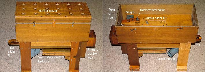
Simulation of wind supply with an air dump tremulant

by Johan Liljencrants

A classical air dump tremulant, in the form found in Wurlitzer theatre pipe organs is described. An attached special purpose Windows PC program simulates its acoustic network. Here several design and adjustment parameters can be interactively manipulated, leading to detailed computed pressures and airflows throughout the system. This may be an aid to understand and master a trem installation. You can also study the dynamic effects from the supply trunk when playing with the tremulant turned off.

Introduction

The tremolo effect, a periodic modulation of amplitude and frequency, is done in a pipe organ by modulating the wind chest pressure. The device for this purpose is called a tremulant, colloquially a trem. The primary goals for trem adjustment is to set a proper rate, typically around 7 Hz, and depth, the relative variation in pressure. Other requirements are that the effect should start smoothly when turned on, and that it should not be too influenced from the number of simultaneously speaking pipes on the chest.

A common trem implementation  is a self-oscillating bellows and pallet mechanism, connected by a trunk to the wind chest. When this mechanism operates it dumps periodic puffs of air from the chest. This type of tremulant is notoriously known to be difficult to adjust, and is also somewhat wasteful with air supply. Because of this, naturally, several competing principles for tremulants exist in the organ world.

One part of the problem to install a trem is to decide dimensions of trunks and bellows, another is to set its adjustable valves and weights. The present simulation may be a support, both in planning and maintenance work.

A Wurlitzer tremulant


Fig 1. A small Wurlitzer tremulant. Left complete, right with muffler cover removed.

The tremulant mechanism proper is enclosed in a box where input air is connected at the bottom, where an input slider sets an input aperture. The mechanism, detailed below, is normally covered by a felt filled muffler with several exhaust holes on top. This is to attenuate the periodic noise bursts coming from air escaping from the output slider. Below the trem box is a control machinery to turn the trem on or off. This is in form of a magnet valve, a primary valve, and a comparatively large secondary control bellows.
 

Short description of the trem function

With the bottom control bellows inflated the mechanism is at rest. Then the upper bellows lid is lifted and the pallet is held closed such that no air can enter at the trunk connection.

To start the tremulant the control bellows is evacuated. This allows also the upper trem bellows to collapse from its own weight and the pallet will begin opening. As the pallet opens there is an increasing flow into the bellows. The ultimate flow is however not limited by the pallet, but is restricted by the aperture of the input slider. 
  
   Fig 2. Simplified drawing of the trem interior.

The flow rate and the aperture of the output slider define an internal pressure Pb gradually building up. When this pressure is large enough the bellows is inflated again, driving the pallet to close eventually. When this happens there will be a temporary peak in the input pressure Pt by the 'hydraulic hammer' effect from the flowing air column in the trunk being abruptly stopped as the pallet slams shut. This pressure peak is higher than the supply pressure to the organ. After some time this pressure pulse will die out and we are ready for another cycle where the bellows can collapse again from its own weight

Measurement on a physical unit


Fig 3. Measured pressure waveforms in a small Wurlitzer tremulant.
The waveforms of fig. 3 were measured individually with a pressure transducer on a small Wurlitzer tremulant, supplied from a 50 mm dia. tube, 2 m long, connected directly to a fan. Their relative timing is not warranted, but a few preliminary observations can be made.

The pressure Pc at the feeding end of the trunk oscillates reasonably around the about 3.6 kPa (14inWC) supply. Not much can be said about the magnitude of the variations since nothing is known of the feeding impedance.  The Pt trace at the input of the trem, at the opposite end of the trunk, shows very large variations, from very low up to about twice the supply. This demonstrates the 'hydraulic hammer' effect and suggests that the trunk has a profound effect on the trem function. The pressure difference across the pallet varies very much. As a contrast Pb inside the trem bellows is always very low, maybe to a surprise, nowhere near the organ operating pressure. With its fairly large lid area, little pressure is needed to raise its weight.

Analog circuit for simulation

For simulation of the system an analog network was developed as in fig. 4. Left is a stylized drawing of the physical system with relevant dimensions indicated in green. Blue symbols indicate pressures at a few places.

The correspondent analog diagram is shown at right. This has symbols borrowed from electrical technology, though all its elements in our case are acoustical. The purpose of that diagram is to formalize which ways the different airflows U will take, and to visualize how you can compute partial pressure differences from the flows passing the various impedance elements, denoted in black. The most basic method here is to apply Ohm's law in acoustical terms. This law is Pressure=Flow*Impedance, in analogy to the electrical case where Voltage=Current*Impedance. For an interested reader further technical detail is developed in the appendix below.

All is driven from a supply regulator by the pressure Po which is taken to be constant. An airflow Ur is fed by a trunk of length Lr and diameter dr to the wind chest of volume Vc. Ao is an open area from the chest representing the flues of any speaking pipes that together consume flow Uo. Uc is the flow taken to compress the chest volume of air in case its internal pressure Pc should vary. The next trunk of length Lt and diameter dt is terminated at the trem input slider of area A1. The product of pallet opening h and length Lb represent the pallet opening area. The smaller of this and A1define a resistance R1 against flow U1 to enter the trem bellows where pressure is Pb. A2 is the area of the trem output slider, with R2 taking the output flow U2. The mass mb and area Ab of the bellows result in an inertial element Mb, and in the same time contributes to a counter pressure Pa. Pallet excursion h is computed from Ab and the time integral of Ub.
  

Fig 4. General layout, symbols, and analog acoustical circuit for the trem system.

Simulation program

The attached Windows PC simulation program (tremsim.exe) was written in Borland Delphi Pascal. It presents a screen with numerous scrollbars at the left side, where you can input physical dimensions. With radio buttons you can select whether to see these inputs in SI units or in traditional US, but computations and result reports are done in SI throughout. In the middle of the screen fig. 4 is reproduced as an orientation aid. It is supplemented with resulting values of those impedance elements that are constant, essentially the masses and compliances. The resistance elements vary nonlinearly with flows throughout the simulation time span, which is 1.5 seconds. The nonlinearity in itself could make simulation next to impossible, but this problem is circumvented by a simple minded approximation explained below. At top is an image area to show results as graphs vs. time for the various pressures and flows. Here the zero line and scale can be adjusted with scrollbars. Check boxes at right are used to select which data to display.

Disclaimer: The results of this simulation are believed to be reasonably accurate in quantity, but cannot be guaranteed. In assessing element values for the simulation, the formulas used are in their most basic form, taken from the classical literature, like eqs. (3) and (6) - (8) below. More refined side effects are not accounted for, e.g. like end corrections or bends in a trunk. The discrete time simulation method in itself is approximate, and finally there is some risk from mistakes by the author.

The reader is encouraged to run the program, to modify input dimension parameters at will, and to look at the various result graphs to familiarize with the trem operations.

trem5.gif
Fig. 5. The tremsim.exe screen with settings like for the unit of fig 1, with the Play function checked.

downtrems.gif

Normally the A0 parameter is zero, disregarding what the scrollbar says, no air is consumed from the chest to play any pipes. This changes when you check the Play box beside. Then, in the time interval from 0.5 to 1.0 seconds, the scrollbar value for A0 open area takes effect. This is to show pressure drop and other things change when the chest is temporarily loaded. You can use this button to see what happens when playing, also when the trem is not used. The natural way to turn the trem off is to pull the mb parameter down to zero.

trem6.gif

Fig. 6. Example of playing with the trem off, cutouts from the screen. The trunks and the chest form a Helmholtz resonator that is excited by the changes in pipe flow Uo.

Fig 6 is an example of what happens to chest pressure when trem is not used. This is characteristic of all organs and is sometimes described as 'the life' of the organ. The classical way to hear it is to continuously play a treble pipe, simultaneously hitting a series of staccato chords in the bass. The induced pressure variations in the chest will then cause the treble pipe to twitter (=tremulate). In classical organ building there is a common recommendation the trunk from reservoir to chest should be made wide and short in order to minimize this effect. But in case you do so, this is counter productive when connecting a trem.


Discussion

In an existing installation most parameters like trunk and trem bellows dimensions are already given. Then you can examine what happens when changing the parameters A1, A2, and mb supposed to be the normal parameters for an adjustment.

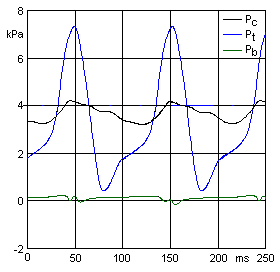
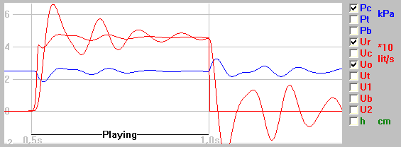
The net airflow consumption of the trem is U1 which has a waveform typically reminding of half sinusoids, skewed to the right. This excitation shape is typical for many airflow interrupting devices like reed pipes, diaphones, orchestral reed and brass instuments, and the human glottis. Indeed the whole trem system can be likened to a diaphone pipe, blown backwards from its mouth at the supply regulator. Like in the mentioned examples the pulse flow from the interrupter is connected to a resonator, in our case the trunks and the chest, to produce an amplified flow oscillation Ur at the mouth, and which may reach quite high values. It should be noted that part of a trem cycle this flow may go backwards to refill the regulator. The regulator is supposed to deliver a constant pressure Po. Even when it manages to do so, its bellows lid will oscillate because of the alternating Ur.
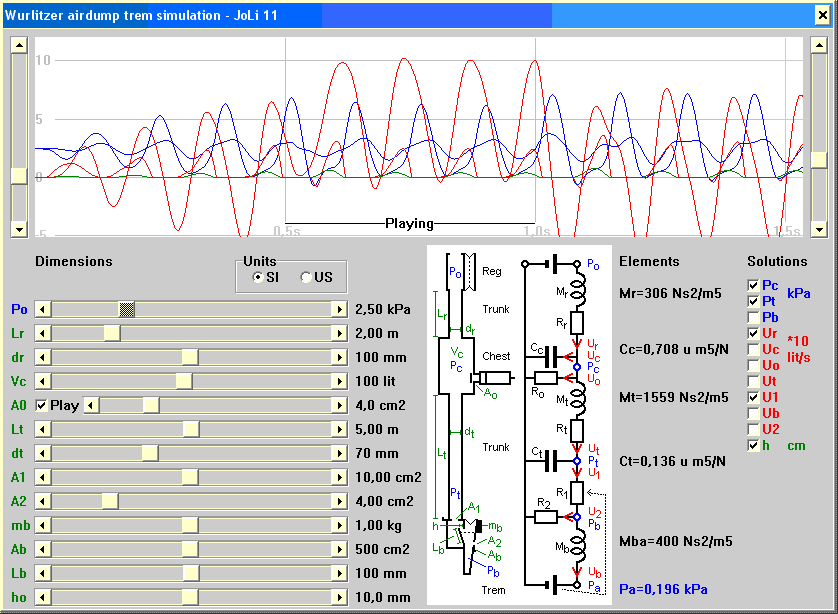
Example calculation: With Ur about sinusoidal 100 lit/sec peak/peak at 7 Hz, then the volume displacement in the regulator will be U/(2π *f) = 100/(2π*7) = 2.3 lit p/p. That renders a lid oscillation about 6 mm p/p when the lid area is 0.38 m2.

The regulator in this simulation is assumed to be perfect in delivering a constant driving pressure. A practical one may vary somewhat in static output with its reservoir fill, depending on how its bellows and spring/weight load match. This is a problem that has minor influence, not accounted for here. A decently constructed regulator usually holds its static pressure within few percent. The initial version of this essay has received some criticism because of this assumption that consequently excluded the regulator from the simulated network. The reason to exclude it is that otherwise the total number of parameters would tend to be too high to handle. The assumption is generally good as long as the pulsating flow Ur is not big enough  to make the bellows bottom out. However, after finding a working parameter set for the trem and you know Ur, then it is wise to run the accompanying regulator simulation program to check how it can handle that flow.

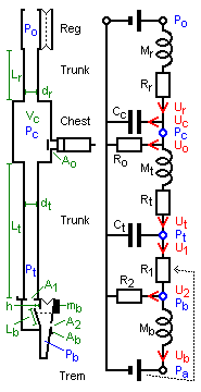
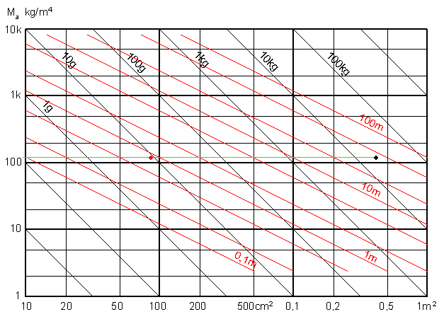
A different thing is the important one, namely the inertia of the regulator. This is its acoustical mass which is found from bellows lid area and weight, including ballast if any. Knowing these data you can account for its effect by adding it to Mr by an increase in the trunk length Lr.
Example calculation: With a regulator lid weight m = 15 kg, area A = 0.38 m2, its acoustical mass is M = m/A2 = 15/0.382 = 104 Ns2/m5, about one third of Mr in fig 5. You can account for that by elongating the trunk about 0.6 m.

It is important to understand this equivalence between regulator lid weight vs. regulator to chest trunk length. Both have the same effect to swamp regulator action what regards changes in airflow, but little concerning static conditions. This is further elaborated below in the technical section about trunks.

Following the lid, the regulator input valve will oscillate. This will partly invalidate the reasoning above, since regulator flow is not only its lid displacement flow, but also refilling flow pulses. However this generally has a relatively minor influence on regulator output, even when its upstream pressure varies considerably.
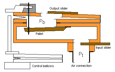
The pressure Pt at the trem input varies much more than the chest pressure. There is a sharp pressure rise when the pallet closes, the hydraulic hammer effect, an expedient to keep reliable oscillation. It is noteworthy that the diameter dt of the chest to trem trunk is of some importance here. If you make it too large, then the linear air speed corresponding to Ut will be small, reducing the hammer effect.

The trem input slider A1 limits the exciting U1 pulses and often appears useless, having little effect until you make it rather small. It is sometimes left wide open to allow for maximum pipe load which is controlled by Ao. If used the trem function may deteriorate unless A2 is fine adjusted.

The useful part of the trem flow is Uc that compresses and rarifies the chest volume, producing the desired modulation in Pc. Knowing a quarter wave resonator for 7 Hz to have a length about 12 m, it is tempting to expect this to be an optimal Lt. The trem trunk would then be assumed to be an isolated resonator amplifying the pulses into the chest. This is not justified, because the other resonator components are firmly coupled. Together they force a much lower resonance than for that trunk alone. This is also evident from that tremulation rate is similarly influenced by the several parameters Lr, drLt, dt, and Vc. This ensemble of parameters together control the resonance of the trunks and chest. For efficiency and clean operation it is desirable that this resonance is close to the tremulation frequency. Just as with any reed pipe there should be a match between resonator and exciter where mb is a key parameter.

Also, the inertia from Mr of the supply trunk is a valuable obstacle for flow oscillation to reach the regulator. The length Lr of the regulator to chest trunk, augmented for any weights on the regulator lid, is a prime parameter to control the depth of the tremulation. It is useless and wasteful to connect the trem unit directly to the regulator rather than to the chest. The chest pressure variations would then become small, to the extent the regulator can do its work. For efficiency in the trem it should connect to the chest as done here. The regulator to chest trunk should be sufficiently long, and as narrow as possible without starving necessary feed to the chest. Then a major portion of the oscillationt of the flow induced by the trem will remain in the chest, not so much of it getting lost upstream into the regulator.

Several, if not all parameters have limited ranges outside which the trem device no longer works. These ranges are defined by usually several of the other parameters. To take a simple example, the supply pressure Pr together with pallet dimensions and trem bellows area set a lower limit for the bellows weight mb. This must be large enough to open the pallet against the supply pressure.

A main purpose behind this simulation is to show how total performance is modified, whichever parameter you select to change. But, despite this simulation uses scientific methods, the experimenter should be aware of the proverb:
To control a system with more than six parameters is art, not science.


Appendix: Simulation procedures 

The following section is highly technical and is probably interesting only to a reader familiar to circuit theory.

Initially at time zero all variables are known, pressures either Po or zero, all flows are zero. From all the known elements and variables an equation system is set up, using an extended variant of Ohm's law, namely the Kirchhoff laws:
 - Going around each mesh in the network, the motive pressure equals the sum of flows times impedances.
 - For each node the sum of entering flows is zero.
This rendered five mesh equations and two node equations for this network, excluding the almost trivial one with pressure Pt. In total a system of  7 equations for 7 unknown flows U, illustrated in Tab.1 below. The equation system is then solved using a standard Gauss-Jordan algorithm. From that all the flows U become known, and it is simple to update the pressures Pc, Pt, and Pb, directly from eq. (2) below. It would work just as well to include these pressure expressions as part of a bigger 10*10 equation system, but the solution algorithm would then take some more time to perform.

Had all parameters been constant and the elements been resistive, then this result would have been stationary and final. But this is not case since the pressures across the reactive M and C elements depend also of time. The impedance expressions for reactive components contain time derivatives or integrals of flow. So the basic principle used here is time stepping with a small time interval τ.

For an acoustic mass the pressure across it is mass times the time derivative of flow, P=M*dU/dt. That is here approximated in difference form as
P = M * (U - U) / τ           (1).        
The strikethrough denotes the known value from the previous computation round, so the time derivative is taken as
(change in flow)/(time step).

In the same spirit, for a compliance element C the integration of flow U renders a pressure across it
P = P + U * τ / C .            (2)
During the time slot a small volume U * τ enters the compliance element. Dividing this by C gives the corresponding increment in pressure, adding to the hitherto existing pressure P .

The solution gives new values for the U and P variables, valid for a new time, one interval τ later. Having come that far all resistances R are re-computed, based on flow values from the previous step, now labelled U . The 7 equations thus contain several values of P and U , known from the previous computation cycle.

This cycle of setting up the equation coefficients and solving is iterated, keeping record of the sequence of solutions for display afterwards. When any of the input parameters is changed, the program runs 768 iteration cycles with τ = 0.002 sec to cover the waveform development from start to just over 1.5 seconds. Such an entire round is computed in a small fraction of a second.

Eq
Unknowns
Knowns
#
*Ur *Uc *Uo
*Ut
*U1
*Ub
*U2
  =
1
Mr/τ+Rr τ/Cc


Po - Pc + MrUr
2

-τ/Cc Ro


Pc
3


-Ro Mt/τ+Rt+τ/Ct -τ/Ct

MtUt/τ - Pt
4


-τ/Ct τ/Ct+R1

R2
Pt
5


Mb -R2 MbUb/τ - Pa
6
-1
+1
+1
+1


0
7


-1
+1
+1
0

Tab. 1. The seven network equations used in the simulation, displayed in a matrix like way. Eq. # 1-5 are branch equations, # 6-7 are node equations.
Clarifying example: Fully written out eq #5 for the last branch would read 
(Mb/τ)*Ub - R2*U2 = MbUb/τ - Pa ,
which is rearranged from the original equation, going clockwise, in form  Mb*(Ub - Ub)/τ - R2*U2 = - Pa .


Acoustical elements

The three basic element types are resistances R, masses M, and compliances C. The following describes how these are handled in the simulation. SI units are used throughout this section. The air properties are taken as:
ρ = 1.2 kg/m3   density,
c = 343 m/s      speed of sound.

Resistances R

A flow U through a linear resistance R develops a pressure across it: P = R * U. A major difficulty in the current problem is that the resistances are non-linear, the resistances themselves are functions of U. This makes it impossible to solve the system equations accurately unless you resort to iterative methods. Since this would complicate simulations beyond reason a simple minded approximation was used, namely to estimate resistance values for the next time step using the past, already known U. Often this works well, when flows do not change appreciably from one time slot to the next. But this is not always true, in particular when the pallet closes, so occasionally this can make computations break down from instability. The remedy here is to average also a newly estimated R with its previous value R. Special care must be taken when an aperture area approaches zero, the resulting resistance is then forced to a large, but finite value.

Two kinds of resistance elements are encountered:

Resistance of a constricting orifice.
This applies to the pallet and the adjustment sliders. With flow U through area A, the Bernoulli law tells the pressure drop
P = 0.5 * ρ * ( U / A )2.          [Pa = N/m2]       (3)
This renders a resistance
R = P / U = 0.5 * ρ * |U |/ A2   [Ns/m5]            (4)

Since resistance is positive, irrespective of flow direction, it is important to use the absolute value |U| of the flow when a resistance is estimated this way. Otherwise the resistance would become negative, should flow direction reverse. Such non-physical behavior would cause collapse of the simulation.

Resistance in a trunk.
This applies to the chest and trem trunks. From a classical HVAC engineering diagram of pressure drop per length vs. flow and diameter I arrive at the approximate empirical formula
R = 0.0244 * L * |U| / d5                                    (5)

It may be interesting to note that for a trunk, 40 diameters long, the orifice and trunk formulas give the same result.
 

Masses M

The acoustical mass of air in a trunk is
M =  ρ * L / A       [Ns2/m5]                                (6)

The mechanical mass mb [kg] of the trem bellows lid, having the area  Ab [m2] is converted into acoustical mass by
Mb = mb / Ab2       [kg/m4 = Ns2/m5]                   (7)

Compliances C

The acoustical compliance of a volume V is
C = V / ( ρ * c2 )   [m5/N]                                    (8)

Trunks

A trunk is a transmission line, generally represented in network theory with a chain of links. Each link has a series M component and a shunt C component for a corresponding lengthwise segment of the line. They are possibly supplemented with resistance elements to account for losses, as done here with Rr and Rt. M and C are computed for the air enclosed in a segment as in eqs. (6) and (8) above. In this simulation the shunt C element of the supply trunk is not visible in the diagram, it is taken to be a minor additive part of the chest compliance Cc.

This representation is valid for low frequencies only, a segment should be shorter than a quarter wavelength in the signal transmitted. In this simulation the trunks are represented by only one single MC link each, and the maximum length you can set is 10 m. In that extreme case the critical frequency comes down as low as into the 10 Hz range, so waveform details are then not overly reliable.

acoumassx.gif
Fig 7. Nomogram to determine acoustical mass from eqs. (6) and (7). The red lines apply to the length of a trunk, the black to the mechanical mass of a bellows lid. The two example points show that the acoustical mass of a 20 kg bellows lid of area 0.4 m2 is the same as for a trunk of 10 cm diameter and length about 0.9 m.

The pallet

To handle the pallet requires a few tricks, additional to the problem of estimating its flow resistance R1. The pallet opening h is found from integrating the flow Ub into the trem bellows. When h goes down to zero the lid motion is abruptly stopped. In the simulation then Ub is then forced to zero, with no further care of any mechanical side effects, like e.g. a bounce against the seat. The expedient to eventually open the pallet is the pressure Pa derived from the lid weight and area. This term enters at the right hand side of eq. # 5 in Tab.1. This is additionally corrected for the opposing pressure difference Pt-Pb operating across the pallet. The correction is that difference, geared down by the factor 0.25*Lb2/Ab. That is, pallet area divided by bellows lid area, and where the pallet width is arbitrarily assumed to be one quarter of its length.

The parameter h0 is maximal pallet opening, where the them bellows is collapsed. This represents how the bar is set, joining the lid and the pallet. This parameter is of no concern when the actual pallet excursions are less, which is the normal case. The only action taken for h0 in the simulation is to zero the trem bellows driving pressure Pa, should h > h0.


2009-02-15, rev 2011-11-02