What size of an organ fan?

by Johan Liljencrants

A recurring question is how much of a fan or other air supply you need to keep an organ fully breathing. There are recommendations on this in catalog data from leading organ suppliers, formulated in terms of airflow and drive power per pipe rank, at different pressures. However recommendations differ substantially between sources. Here is a discussion around this, reasoning from basic physical laws. First about what a blower fan can supply, how pressure depends on diameter and speed, and that airflow depends on cross sectional area. Second, what an organ performance consumes, in regular playing as opposed to thundering chords. With a conservatively over dimensioned fan supply you run the risk of the air to be excessively heated. It is proposed that conventional fan supply is surpassed by old fashioned feeder bellows, powered by a variable frequency drive.

Air supply

Function and pressure in a centrifugal fan

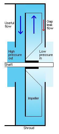
Axial (propeller, turbine) fans produce much flow, but also noise, and typically give nowhere near enough pressure for an organ. We dismiss this fan type from the discussion and concentrate on the centrifugal fan in which a housing encloses a rotating impeller with vanes. The housing has an air intake near the hub of the impeller and an output port near its periphery.

These vanes make the air follow the impeller rotation such that air is pressed toward the periphery by centrifugal force. Based on the basic centrifugal force formula G = m ω² r (force G, mass m, angular speed ω, radius r) you can set up an integral for the pressure buildup from impeller hub out to perihery. Omitting tedious computational detail the integrated result comes out as a pressure P_c = ρ s²/ 2 (air density ρ, impeller periphery speed s). Now, additional to this pressure rise, the air in the housing outside the impeller also has received a tangential speed of the same magnitude s. If you block the fan output such that there is no airflow, this stagnation invokes an additional pressure rise of about the same magnitude P_c, but this time because of the Bernoulli relation between speed and dynamic pressure, see below.

The approximate rule-of-thumb result is that the pressure produced at zero flow is 2P_c = ρ s². This very simple formula is shown in Fig 1 where s is derived from impeller diameter and rotational speed.

fan pressure vs speed and diameter

Fig1. The vertical scale is for the benchmark static pressure obtainable from a single centrifugal fan, given rotation speed and impeller diameter.

Pressure is proportional to impeller diameter squared

Pressure is proportional to impeller RPM squared

This is the stagnation pressure you can expect from a centrifugal fan, the pressure when output is blocked and no flow is taken out. A first point is that this pressure is linked to the diameter of the impeller and its rotation speed. Engineering inventions like shaping the rotor blades can change it to some degree from the indicated value, but not very radically. Textbook knowledge says that forward swept blades increase pressure, backward swept lower it when flow increases in the low flow region.

If you limit diameter (to keep space down) and speed (to keep noise down) the only remaining option to elevate pressure is to put two or more fans in cascade, one driving the next. Unless you use a belt drive, with common AC motors there are normally only two options for the speed, either 'low' 1400/1700 or 'high' 2800/3400 RPM, depending on motor design and whether you have 50/60 Hz mains.

Dynamic pressure

Because of its formal likeness we may at this point recall the concept of dynamic pressure. This is one of the terms of Bernoulli's equation, which is essentially an equation of energy conservation for a fluid in motion. The dynamic pressure is equal to the difference between the stagnation pressure and the static pressure. Static pressure can be identified for every point in a body of fluid, regardless of whether the fluid is in motion or not. It can be measured using an aneroid, a U manometer water column, or various other methods.

The fundamental Bernoulli law tells the dynamic pressure in relation to air speed:

P_d = ρ*v²/2 = ρ*(U/A)²/2, where

P_d is the dynamic pressure in Pa = N/m²,
ρ is the density of air, ρ = 1.2 kg/m³,
v is the linear air speed in m/s, which in turn can be written as U/A, with
U being the flow rate in m³/s streaming through an area A in m².

One application of this law is that it tells at what speed v and flow U air that will emerge from an open area A in the wall of a container holding the pressure P_d. For instance, this tells speed and consumption in the air jet that excites an organ flue pipe. These and related quantities are illustrated in the diagram of fig 2.

Another application relates to the stagnation pressure delivered by a centrifugal fan when its output is blocked, as mentioned above.

The dynamic pressure is also a primary guide to find the aerodynamic force on a body in an air stream, or with the body moving through still air. The general procedure is then that you estimate the force as the dynamic pressure times the body area. On top of that you will have to apply an empirical correction factor that applies to the specific body shape. This drag coefficient is generally not far from unity.

Fig 2. Physical parameters related to the Bernoulli law. The vertical scale is for dynamic pressure and at left is a scale for the corresponding linear air speed. Horizontally is flow. The graph surface tells in blue the constricting area necessary to let through that airflow when you exert the pressure across it (flow U = vA, speed times area), and in red the power released in the process (power W = UP, flow times pressure).

Example of how to read. Across an opening of 10 cm² (blue line) you exert a pressure of 1 kPa, or 4 inWC (right scale). The resulting air jet speed is then 41 m/s (left scale) and flow is 41 l/s or 88 CFM (bottom scale), while the power expended is 41 W (red lines). If you raise the pressure fourfold, then speed and flow will double while power increases eightfold.

Some use of the fig 2 diagram is shown with practical fan data below. We will also return to this figure with relation to organ air consumption.

Practical fan examples

Fig 3. Data sheet for a medium pressure industrial fan with swept back impeller blades, adapted from http://www.ventur.se.
In fig 3 the upper graph at left shows the static pressure at no flow to be 3.3 kPa. This is somewhat less than the idealized 4 kPa prediction of the diagram for a 0.4 m dia impeller at 2800 RPM. When you begin to draw a flow the total pressure remains at first, actually rises a little despite the blade back sweep, but at heavier load it drops off steeply. The lower graph shows the dynamic pressure, increasing with the square of flow. For this particular fan the two graphs meet at 680 lit/s and 0.58 kPa. This comes when you run the fan alone, with nothing connected. Then there is no static pressure difference between its input and output, all effort is used to accelerate the air leaving the output. When you locate this point in fig 2 you can read from the sloping lines a constriction area of 210 cm² and a power of 400 W. That power represents what is expended to accelerate that 'short circuit' airflow through the fan, but it does not include a large number of other power consuming phenomena like viscosity and turbulence losses in the air stream, and whatever mechanical friction losses. The 2.2 kW installed motor power is just over twice the delivered air power in the useful range. The area indicated is a trifle larger than the open area of the connecting ducts which suggests that the fan interior is fairly well streamline shaped. Though this extreme running condition is of little practical interest it still has a value in pointing to that flow capacity is limited by the cross sectional area of the internal air path of the fan. The pressure difference between fan output and input is the difference between the two graphs of fig 3, left. The illustrated example fan could perhaps be used for an organ up to a flow rate of 250 lit/s (900 m³/h, 500 CFM). Within this flow range the output pressure essentially remains and the dynamic pressure is negligible by comparison.

		Fig 4. Data sheet for a two stage Ventus blower, adapted from the Laukhuff catalog.
The data sheet of fig 4 is one of very few I have seen published on dedicated organ blower fans. It is for a two stage, high speed, high pressure unit. Again, from fig 1, to get half the no load pressure from one stage at 2800 RPM would require an impeller diameter approaching 0.3 m, which appears plausible from the drawing. At the maximum rated flow 75 lit/s (160 CFM) the 67 cm² output area would render a linear air speed about 11 m/s and a negligible dynamic pressure about 75 Pa (0.3 inWC).

Trunks, grooves, and valves

The cross section of connecting trunks should match the fan to ensure that the linear air speed inside corresponds to a low dynamic pressure, as compared to the working static pressure. The ultimate use for the blowing air is to have it accelerated in the pipe flues to produce the oscillating air band that excites the pipes. Here again the Bernoulli law comes into use, telling the relation between the air band speed and the foot pressure in the pipe, again this speed is flow divided by the flue area. To keep foot pressure near the rated pressure it is necessary that there are no essential constrictions for the flow on its way there. A handy rule may be that any flow constriction on the way to the pipe flue, like in a valve or a foot hole, must have at least 3 times the area of the flue itself. That would then leave about 90% of the nominal pressure across the flue aperture while 10% are lost in the constriction. A conservative builder would use larger air transport areas than that in order to preserve pressure to the pipe.

Conversely, in some voicing work constrictions are deliberately introduced, usually by control of the toe hole diameter or some other obstacle in the pipe foot. The purpose is then to lower the pressure drop across the flue, the air band speed, and the sound power from the pipe.

Fan shortcomings

It happens that a plain vacuum cleaner fan is suggested, and even used for an organ application. Such a fan is driven by a series magnetized commutator motor, the characteristic of which is that its speed goes down when load increases. To use that in an organ should be discouraged for several reasons. One is that pressure varies widely vs. flow consumption. When the organ pauses and little flow is drawn, then because of the lower load the motor speeds up to make more noise in the same time as pressure increases beyond reason. A special spill valve is desirable to limit this and to insure motor cooling. It puts hard requirements on a pressure regulator, and when you pass the limit of what flow can be supplied, then pressure drops steeply. Unless you arrange for a separate cooling path for the motor the soot released by the motor brushes will also contaminate the organ interior.

Efficiency

An ideally efficient fan would consume drive power in proportion to what is delivered. The output air power W watts is the product of pressure P in Pa times flow U in m³/s, W=PU. When blocked to zero flow, no useful power is produced. But the motor still consumes power because of a number of loss mechanisms, one of them is the turbulence created. Occasionally data on the fan efficiency are published, i.e. the air power delivered, divided by the power to the drive motor. Typically the point of best efficiency comes at a flow about half the free blowing maximum rate. Moreover this efficiency is rarely much over 50%. On average an organ blower delivers much less than this optimum flow, but motor power still does not decrease appreciably. A major part of the power supplied to the motor then goes to heat the air rather than to drive the music.

Heating

An important part of this loss is sometimes mentioned in passing, but without any numbers, namely the leakage from the pressure side back to the fan input. Fig 5 sketches a typical situation, showing one stage in a classical Spencer Orgoblo fan. The low input pressure is elevated by the impeller rotation. First notice is the fact that the compression itself will heat the air about 1 degree centigrade for each 5 inch of water column pressure rise. This small temperature elevation is a consequence of the general gas law.

However, the clearance gap between the fan housing and the impeller leaves place for an undesired and highly turbulent back flow (red arrow in fig 5). As an example, in the Orgoblo manual a clearance of 3 mm (1/8") is recommended (other sources say even more, up to 1/2"). This would present a return leakage area to the order of 30 cm² and a flow of 250 l/s drawing about 1kW at 4 kPa (15 inWC) pressure. This power is dissipated in turbulence and acts to progressively heat the air as it circulates internally, inside the fan shroud. Theoretically then at a rate of 3 degrees centigrade per second. If you draw little flow from the fan this is a significant heating agent, even if the practical heating rate will be much slower because the heat is distributed into the mechanical structures of the fan..

Working in hot climates people have cooled too hot organ air by water injection, which is potentially an organized organicide. This problem will increase when a fan installation is over dimensioned in order to safeguard against lack of air.

It is indeed lucky that a silent organ is not airtight, there are all kinds of ways some wind will escape through wood, leather, cracks and slits. This total leakage flow is mostly quite substantial, it is often comparable to the flow to the pipes at average playing. It represents power lost, but the good side of this is that the turnover of air keeps the temperature rise within limits.

Fig 5. Internal fan leakage

With a myriad of parameters a further theoretical analysis would appear fruitless, but the following may guide the control of heating in a prospective or an existing fan installation. Block the the intake or the outlet of the fan, whichever is the easier. Then run it for a limited time while estimating the electrical power fed to its motor. This way of running a fan is sometimes discouraged, precisely for the reason that for lack of cooling it will overheat with time. The power may be estimated with an ampere meter, but then you must also multiply by the cos(Φ) power factor, number of phases, and voltage. A perhaps better alternative would be when you could use the mains elecricity meter, subtracting whatever other loads that may be connected to it during the test.

All of the power W [kilowatt = kJ/s] determined this way will go into heating the air and the fan. Now, knowing that the heat capacity of air is about 1 kJ/(kg*K) and air density 1.2 kg/m³ we can compute a minimum flow rate U_min m³/s necessary to keep a specified maximum temperature rise T_max in centigrades:

U_min = W / (1.2 * T_max)

For example, if the blocked fan consumes W = 1.2 kW of power and we allow the air temperature to rise at most T_max 5 degrees centigrade, then the flow through the fan must be at least U_min = 0.2 m³/s.

Variable Frequency Drive

In power saving schemes for pumps the use of a Variable Frequency Drive (VFD) is often proposed. With organ blowers we want constant pressure, hence also require essentially constant motor speed, so here the variability aspect is not an interesting issue. If you reduce speed, even moderately, then the regulator pressure margin may vanish such that blowing pressure is not upheld. But in case the fan delivers a pressure that is notably higher than necessary, then you can reduce power, heating and noise by using a VFD set to run the fan constantly at lower speed than its nominal. This is a primary merit of using a VFD, together with its ability to convert the power 'format' if necessary, e.g. to drive a three phase motor from a single phase mains supply.

However, in case the fan or the trunk from fan to reservoir has too low capacity, such that pressure is not upheld at large demands, then a VFD can help somewhat by trying to accelerate the fan. The problem is then to derive a good control for the VFD. Classical control is taken from the elevation of a reservoir lid, but in view of the large inertia of a fan it would be better when you also could directly detect increase in flow consumption.

Ways to avoid the air heating problem are costly, one way or the other.
- Use a precision fabricated high efficiency fan where the shroud-impeller clearance is very small. Expensive to make.
- Install a fan of adequate size, with no overkill capacity. A key question, how would you know required capacity before it is too late?
- When organ air consumption is low at playing intermission, arrange for a spill valve at the fan output to keep up intake of cool air. Pay the power bill.

How to measure airflow

To find the pressure inside a trunk is easy enough, to a probe hole you can connect a U manometer or any other more modern pressure indicator, and this would not disturb the system in any way. Airflow is much more difficult to estimate. Several methods come to mind where you actually measure the linear speed of the air by some kind of anemometer. Knowing that speed you multiply with the relevant area to obtain the corresponding flow, generally assuming that the speed is the same across the area.

A practical problem is that the anemometer should be small enough to fit inside the measurement area without too much pingpong ball
anemometer calibration

interference with the flow, and that its measurement range should be adequate, generally up to perhaps 10 m/s. Perhaps a bowl cross, common with weather stations, would be too big, but there are simple commercially available anemometers using a small turbine, driven by the airflow. A simple low precision device may be a hanging vane or a pendulum, a ping-pong ball hanging from a thin wire is a classical example. Here you can estimate horizontal air speed from the angle the pendulum is deflected away from its vertical rest position, fig 6.

Fig 6. Calibration for a ping-pong ball pendulum anemometer measuring horizontal wind speed. Ball mass 2.7 g, diameter 38 mm. In this air speed range the drag coefficient for a sphere is typically 0.52.

Some anemometers use how the Bernoulli equation relates speed to a pressure drop as the flow passes a constriction in the trunk. The problematic issue is then that to be measurable this drop is generally big enough to disturb the working conditions. To make this method useful the upstream pressure might then be raised in order to compensate for the drop in the measuring device.

See also http://en.wikipedia.org/wiki/Anemometer , http://www.fonema.se/anemom/anemom.html .

Air consumption

How much air for one rank? Legend tells that Bach used to scare organ builders by pulling all stops simultaneously, to check whether the lungs of the organ could cope. In modern times builders would rely on generally agreed recommendations like the one in fig 7. This suggests the flow required for one five octave rank at different pressures. One rank then means 61 pipes, there are further rules for larger sets, e.g. a 97 note compass could be counted as 2.36 ranks. These data pairs of pressure and flow line up nicely in fig 2, all of them tell that they presuppose that one rank presents an average open area for the wind about 6 cm² (1 sq inch). This area is then the sum of flue areas for simultaneously speaking pipes plus whatever leaks may be present. The recommendation does not explicitly mention rank footage which should be important, but most probably 8' ranks are assumed. As born out below a 16' rank should use twice as much air. A different rule of thumb, supposedly empirical, says that you for theatre organs would need about 10 CFM (5 l/s) per rank at 10" pressure. This is about 8 times less than what is given by fig 7. This rather large discrepancy is the reason the present article was written at all.		Fig 7. Estimated rank consumption (abbreviated quote from the OSI catalog, Arndt gives similar data).
To put this problem into perspective the following is an attempt to estimate more precisely the necessary supply flow, based on physics and statistics. One foundation is then how pipes are typically dimensioned. Another is analysis of how many pipes speak simultaneously in an average musical situation, as a fraction of the total 61 in a rank.

Consequence of equal pipe sound powers

Fig 8. The relative pipe flows in a 'standard' 8' rank of 5 octaves compass, plus the adjacent octaves. Theoretical values, assuming all pipes are equally efficient and produce the same sound power. Bottom are MIDI note numbers and conventional footage designations.		The acoustic power delivered by a monopole sound source, like a pipe mouth, is proportional to the square of its frequency F times flow U. Assume for reasoning that the sound power delivered from each pipe in a rank is to be same. This then means that for each pipe acoustic flow will have to be inversely proportional to frequency. Since all pipes within one rank are similarly built, we can assume their conversion efficiency from wind to sound power is the same. Then also the supply flow and flue area should vary the same way. We may represent this with a proportionality that both of U, A ~ 1/F ~ 2^-n/12, where n is semitone note number on a rising scale, e.g. like MIDI, illustrated in fig 8. Incidentally the same proportionality as for the length of the pipes. One consequence of this proportionality is that the lowest octave in a rank will use about the same supply flow as all its higher octaves combined. Another is that flue area and flow rate for the lowest pipe is 5.6 % of that for a whole 61 note rank, 0.18% for the highest pipe. It should be noted that this scale of halving on every twelwth note is about the power supplied to the pipes. It is a hypothesis drawn from the fact that pipes within one rank are made with a similar construction, and the presumption of their equal loudness.
This is not the same thing, and it does not conflict with the pipe width scaling rule that typically uses a halving number M=18 like in a Toepfer scaling scheme. This latter aims at controlling the timbre and pipe Q values within a rank. E.g. in such a typical rank where width halves on the 18th pipe, then the airband thickness would presumably halve on the 36th pipe. In that case the flue areas will still follow the1/F rule, since the exponent for flue area comes out as -n/18 -n/36 = -n/12.

Measuring a rank

First we could now look at how pipes are actually made. Using a ruler and a feeler gauge, you can measure the flues of one or a few pipes in a rank, the width W of the pipe and the airband thickness D. Flue area is then A=W*D. What concerns air consumption the lower end of the compass is the most relevant. With reed pipes you could take a similar measurement using D for the distance between tongue tip and shallot, and W for the free length of the tongue. Fig 9 shows results of a few such measurements. A first observation is that the hypothesis appears confirmed, that flue areas are really made proportional to 1/F. This follows from that data points within a rank largely line up with the direction of the grid lines sloping at this rate. E.g. the uppermost point in fig 9 is for a Wurlitzer Tibia E (MIDI 52) found to have a width of 57 mm and flue 1.45 mm, a 0.83 cm² area. In the diagram this is connected to the point for the Tibia C (84) having flue area 0.13 cm². A final point for this rank at G (91) shows a slightly larger area than expected. That small pipe is made from metal rather than wood as is the lower part of the rank. Conversely, the variation between ranks may be substantial, in the first place because they are made to produce different loudness. E.g. the principal flute ranks of my own JoLi organ have about half the areas of the Wurlitzer Tibia rank. Also the spread of these data points around the general trend would represent random variations due to amateur construction and voicing.		Fig 9. Individual pipe flue areas vs. notes. Measured data within a rank would fall in the direction of the sloping lines in case individual pipes receive and deliver equal power. The scale at right for these lines indicate an estimate of the total flue area of a standard 61 pipe rank.
In fig 9 the 1/F sloping lines are provided with an area scale to the right. This scale shows the total flue area that will result for a 61 note rank, when its data points fall along the corresponding line. So to estimate this total area you need not measure more than one or a few of its pipes. The exemplified Tibia rank total flue area estimates into 35 cm². This is about 6 times bigger than the 6 cm² area allowed for by the dimensioning rule of fig 7. This should mean you could play at most every 6th pipe simultaneously, if you forget about leaks. Example prospect for my own organ My organ has 247 pipes, organized street organ wise into bass, accompaniment, melody, and counter melody sections, a scheme nowhere near a standard organ philosophy of 61 pipes per rank. But let us assume these pipes represent 4 standard ranks (appr 247/61). Judging from the measured points given in blue in fig 9 we may guess an average rank flue area of 12 cm², rendering a total flue area of 4*12 = 48 cm². At a blowing pressure of 2 kPa (8 inWC) and all pipes speaking simultaneously this would then call for a flow of 270 l/s (550 CFM), according to fig 2. This organ is blown by speed controlled bellows. From its bellows dimensions and crankshaft speed its maximum flow capacity is estimated to be 30 l/s, about one tenth of that total figure. This then means that the supply should be enough to play on average 10% of the pipes simultaneously. However this figure must be reduced by about one third because of the air leakage consumption found when the organ is silent. Still supply appears to be enough, so we can go on relate to the following question.

How many pipes speak on average when you play?

To show what might be musically representative, fig 10 renders analyses from a few MIDI sequences. Most of them are arrangements for my organ, covering a span of 4.5 octaves. The scope is now about the note pattern, it has nothing to do with the size of the organ, such as whether it is registered to use one or forty ranks.

For each tune sample the histogram at top shows for each note the percentage of total time it is turned on. At middle these percentages are weighted by the respective pipe flue areas in proportion to the 1/F rule. At bottom this is accumulated over the compass. The interesting result is now where this accumulation finally lands, the fraction of the total flue area of the rank that is open on average. The accumulation would have been 100 % if all pipes had been speaking all of the time.

This result figure is 3 to 4 % for the first three examples. Since the compass used here is only 4.5 octaves rather than 5, the music may be transposed one half octave down without loss of notes. If you do that the cumulation will increase into the 4 to 6 % range because of the larger weights on low notes.

It is interesting that the end results come out within such a small range, fairly independent of musical style. Probably this is due to the limitation in number of fingers and feet available to a performer. But one should be aware that air consumption would effectively increase by 50 % when you use an octave coupler.

For a long time average the result is in the range around 5 %, one pipe out of 20 is speaking. But consumption will vary around the average. Then comes the task of an air reservoir to enable the winding system to supply a higher flow during a shorter time span, and later refill at less demanding intervals. Now two more questions rise, mutually connected. How much more flow than average must the supply be able to deliver, and for how long duration must the reservoir be able to sustain such a temporary high load condition.

Here it is hard to give any distinct answers. The reservoir providing for short flow peaks to be twice or three times as big as the long time average would cover up a vast majority of cases. One could perhaps prescribe a reservoir volume to keep up such high flow for a duration of, say, 1 second.

But it is easy to figure out a specific situation with high demand, namely a wide final chord with 'full' registration. One such could go on for a long time, certainly more than 10 seconds, enough to exhaust any reasonably sized reservoir. Sustaining a chord with 4 notes per octave in the two lowest octaves will open up about 50 % of the total rank flue area. This by very far exceeds the 'normal' average playing consumption.

Indeed this is a single identifyable condition that sets the limit for what thunder can be produced by the organ.

That tells that the statistical analysis of average air consumption in 'normal' playing is no more than a hopefully stimulating intellectual exercise. And that the organ supply almost all of the time is almost idle, though also feeding the inevitable leaks in the instrument.

Maple leaf rag, Joplin

Tulips from Amsterdam, Arnie-Martyn

La Traviata, ouverture to 2nd act, Verdi

5th symph. Toccata, 24 bars with main theme, Widor

Fig 10. Statistics taken from MIDI files. For each piece the top histogram is the percentage of time each note is on, middle weighted for air consumption, and bottom this accumulated over the compass.

Concluding statements

The static pressure delivered by a centrifugal fan is determined by its impeller diameter and rotation speed, possibly multiplied by two or more cascaded stages. Pressure is proportional to the square of diameter and square of speed.

Since an organ requires a constant supply pressure the fan should go at constant speed. There is little merit in trying to vary fan speed with a VFD depending on required air flow rate, which would anyway be hampered by the big mechanical inertia of a fan impeller. A VFD may however be justified as a means to set a suitable constant speed to the fan and to interface its motor to the available electrical power system.

The maximum fan flow rate is set by its internal cross sectional area, where the output connection flange dimensions give a representative measure. Linear air speed in the flow direction in the fan and in the following trunk system should be low enough that the corresponding dynamic pressure is negligible beside the working pressure, say maybe less than 5-10 % of it.

To estimate the air consumption of a specific rank you can measure the flue area (pipe width times airband thickness) for one or a few pipes toward its lower range. From these data you can estimate the total flue area of the rank using fig 9. This total area may differ significantly between ranks, in the first place depending on how loud they are supposed to be.

The air consumption at 'average playing conditions' is rather independent of musical genre. My analysis finds it to be in the range of 5% of the total rank consumption. Or formulated otherwise, on average one out of 20 pipes is speaking.

The previous statement about average consumption contrasts radically against easily predictable situations like massive final chords, where one could expect ten times more air consumption than average. It is up to the organ designer to decide what should be a maximally allowable registration for a final thundering chord. This appears to explain the vast difference mentioned between various recommendations on supply capacity.

This maximum flow is probably chosen to be several times the average required. This also means that the air supply system on average supplies a rather small fraction of its capacity.

This underlines that a fan should be accurately fabricated, with a small clearance between its impeller and housing. The air circulation inside the fan from its pressure side back to the input is a significant agent to heat the air. A method was suggested to determine what minimum flow that should be allowed through the fan in order to limit this temperature rise.

Proposition in view of modern VFD technology

It is suggested that the common practise today with air supply from a fan is replaced by old-fashioned feeder bellows. The novel feature would be that the bellows drive motor is fed from a variable frequency drive, such that drive speed corresponds to the momentary air consumption. This is indicated by the elevation of the reservoir or regulator lid. This will reduce drive power into what is actually needed, it will eliminate the problem of air overheating, and hold down the noise produced by the air supply.

2009-12-06 JL, rev 2011-07-25